Excel Timelines
Excel wasn't designed for making timelines, but why should that stop us? :D In this example, we're going to create a timeline with overlapping dates.
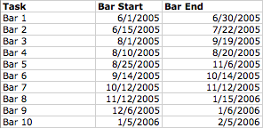
1. Start by entering the dates into your spreadsheet as shown:
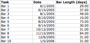
2. Next, subtract the "bar start" values from the "bar end" values to calculate "bar length."
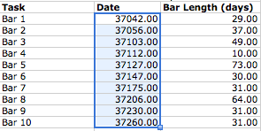
3. Now, Format the dates as numbers (Format/Cells/Numbers...). This is a temporary step to allow Excel to properly graph the data that you will undo later.
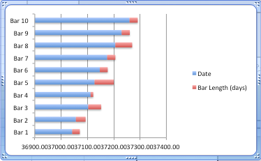
4. Next, highlight your data and Insert a Chart of the type "Bar/Stacked Bar."
5. You can now Format the dates as dates once more in the data column and the chart will continue to work.
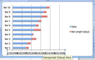
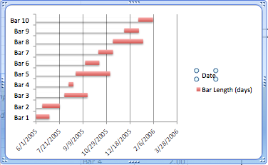
6. Next, double-click on the x-axis in the area where the dates are displayed. We will rotate them to make them more legible.
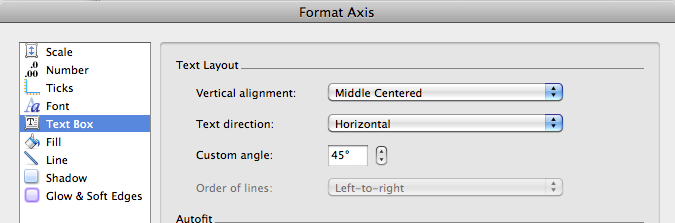
7. In the Format Axis controls, select Text Box and adjust the Custom Angle from 0 to 45 degrees.
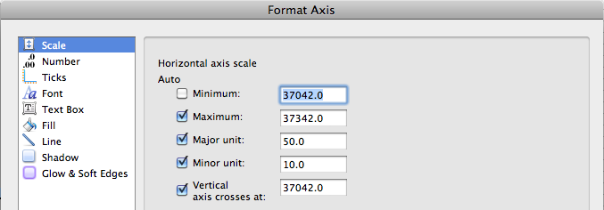
8. Set the scale of the x-axis so that the minimum is the lowest number (the earliest date) in the timeline. In our example, this was "37042.0" which corresponds to 6/1/2005.
9. Now, we need to hide the blue "Date" bars. Double-click on the blue bars or on the "Date" area in the legend to bring up the "Format Legend Entry" controls.
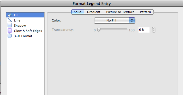
10. Under Fill, in the Solid tab, select "No Fill" from the Color pull down menu and the blue bars vanish!
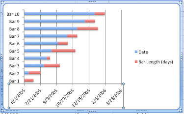
11. Finally, delete the legend itself to cover your tracks! Continue to tweak the chart to get it exactly the way you want it.
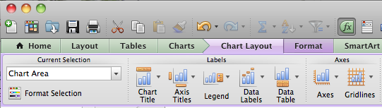
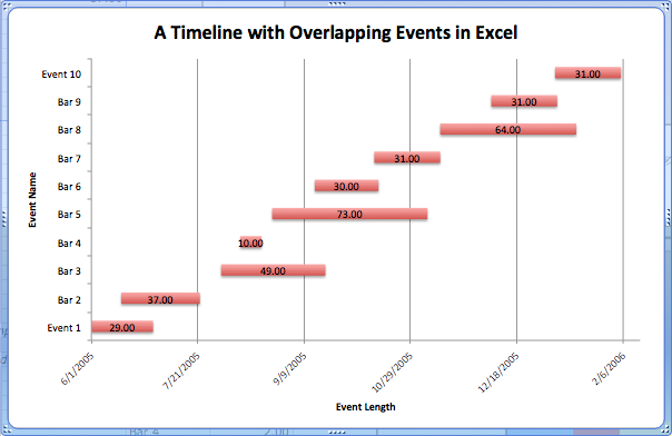
12. Add a title and axis labels from the Chart Layout/Chart Title and Chart Layout/Axis Titles ribbon. Here's a sample of the final product:
13. You can download this example to play around with here. There's also a second, simpler example of a non-overlapping timeline in the spreadsheet.