GRAPH: In this census, the word graph means a simple graph, a collection V of things called "vertices" and a set E of unordered pairs from V; these are the edges of the graph.
SYMMETRY: A symmetry, also called an automorphism, of a graph is a permutation of its vertices which preserves edges. If Γ is a graph, the symmetries of Γ form a group under composition, called Aut(Γ).
Graphs in this Census: This Census concerns graphs of valance (degree) 4 (tetravalent graphs) which are edge-transitive, i.e., those for which, given edges e and e', there is σ in Aut(Γ) which sends e to e'. A dart (or arc or directed edge) is one of the two ordered pairs of vertices corresponding to an edge. If AG = Aut(Γ) is transitive on darts, we naturally call Γ dart-transitive (abbreviated DT); the word "symmetric" is often used with this meaning. If AG is transitive on edges and vertices, but not on darts, we say that Γ is ½-arc-transitive or HT. If AG is transitive on edges but not on vertices, we say that Γ is semi-symmetric, or SS for short.
This most recent edition of the Census, dated September, 2016, contains 3565 DT graphs, 920 HT graphs and 2879 SS graphs for a grand total of 7364 graphs.
The headings in the Table and the spreadsheet version of the Census:
Tag: The tag "C4[20,5]" means this graph is number 5 in the list of graphs having 20 vertices.
V: This is the number of vertices
E: The number of edges
Transitivity or Tr.: This tells which of three kinds of symmetry the graph has. We abbreviate the types DT for dart-transitive, HT for ½-arc-transitive, SS for semisymmetric.
Worthy? or W?: W or U as the graph is worthy or not. (A graph is unworthy if some two of its vertices have exactly the same neighbors; it is worthy otherwise.)
Bipartite? or B?: B or NotB as the graph is bipartite or not.
AG: The order of the symmetry group.
vs: The order of a vertex stabilizer.
ds: The order of a dart stabilizer.
#STO: The nyumber of semi-transitive orientations (see below).
gi: The girth of the graph.
dm: The diameter of the graph
Name: The canonical (i.e., first-encountered) name for the graph. This shows the parameters of one construction for it. Others are listed on the graph's Constructions page.
CIRCULANT GRAPHS: The circulant graph C_n(S) is defined for any integer n at least 3, and every subset S of Z_n which is closed under negation. The vertices are the elements of Z_n, and i, j are joined by an edge exactly when j-i is in S. We usually abbreviate by listing only those s in S which are less than or equal to n/2. Thus K_5 is C_5(1,2). The degree-4 edge transitive circulants are all C_2m(1,m-1) = W(m, 2) and all C_n(1,a), where a2 is 1 or -1 mod n.
WREATH GRAPHS: The vertices of the wreath graph W(n, k) come in n bunches of k each, the bunches arranged in a circle. Each vertex in bunch i is joined by an edge to each vertex in bunch i-1 and bunch i+1. The depleted wreath graph, DW(n, k) is formed from W(n, k) by removing the edges of k disjoint n-cycles. Of these, only W(n, 2) and DW(n, 3) are tetravalent.
TOROIDAL MAPS: There are three families of maps of type {4, 4} on the torus in which the symmetry group of the map acts transitively on the edges. One is the well-known family of regular maps {4, 4}_b,c. These are formed from {4, 4}, the grid of squares, by identifying two vertices whose coordinates differ by an element of the group generated by vectors (b, c) and (-c, b). This map has D = b2 + c2 vertices, D faces and 2D edges. The second is {4, 4}_<b,c> formed in a similar way; the group in this case is generated by (b, c) and (c, b). This map has D_2 = |b2 - c2| vertices, D_2 faces and 2D_2 edges. The third is {4, 4}_[b,c] formed similarly; the group in this last case is generated by (b, b) and (c, -c). This map has D_3 = 2bc vertices, D_3 faces and 2D_3 edges. These maps and graphs were classified by Siran, Tucker and Watkins.
SPIDERGRAPHS: The Power Spidergraphs were named and first investigated by Leah Berman. PS(k, n; r) is defined for k, n, r satisfying rk = 1 or -1 (mod n) but r is not 1 or -1 mod n. Vertices are in Z_kxZ_n. Edges join each (i,j) to (i+1, j±ri). MPS(k, n; r) is similar, except that n must be even and (k-1, j) is joined to (0, j±rk-1 + n/2).
AMC This construction is a special case of one due to Casey Attebury. It is a 2-dimensional generalization of the Power Spidergraph. AMC(k, n, M) has vertices in Z_kxZ_nxZ_n, and M is a 2x2 matrix over Z_n. For i in Z_k and x in Z_nxZ_n, (i, x) is joined to (i+1, x+a_i) and (i+1, x+b_i), where a_i = (1, 0)Mi and b_i = (-1, 0)Mi.
BICIRCULANT GRAPHS: A bicirculant graph is one on 2n vertices which allows a symmetry moving them in 2 cycles of length n. There are two kinds of tetravalent edge-transitive bicirculants. One is the Rose Window graphs (see below). The other bi-circulant graph, BC_n(S), is defined for any integer n at least 3, and any subset S of Z_n. The vertices are all A_i, B_j for i, j in Z_n. A_i, B_j are joined by an edge exactly when j-i is in S. The logo for this Census is BC_7(0, 1, 2, 4). Each BC_n(S) is a Cayley graph of a dihedral group. The edge-transitive ones come in three sporadic cases and three infinite families.
Rose Window Graphs: The graph R_n(a, r) has 2n vertices: A_i and B_i for i = 1, 2, . . . , n. There are 4 kinds of edges:
(1) Rim: {A_i, A_i+1}
(2) Spoke in:{A_i, B_i}
(3) Spoke out:{B_i, A_i+a}
(4) Hub:{B_i, B_i+r}
These are known to be edge-transitive in 4 cases:
(1) R_n(2,1) This is the same as W(n, 2)
(2) R_2m(m+2,m+1)
(3) R_2m(2b,r), where b2 = + or -1 (mod m) and r = 1 or m is even and r = m+1. Exclude graphs in families (1) and (2) from family 3. We separate family 3 into family 3a (where b2 = 1 (mod m)) and family 3b (where b2 = -1 mod m).
(4) R_12M(3M+2,9M+1), R_12M(9M+2,3M+1). Again we separate into two families: 4a is the case where M is odd, 4b where M is even.
Every R_N(a, r) which is edge-transitive belongs to one of these families.
Praeger-Xu Graphs: This is a family of graphs each of which has large vertex-stabilzer. In this Census, we use the name PX for this graph. The vertices of PX(n, k) are all pairs (i,x) where i is a number mod n and x is a bitstring of length k. Edges are pairs {(i,ax), (i+1, xb)} where x is a bitstring of length k-1 and a, b are 0 or 1 independently. PX(n, 1) is isomorphic to W(n, 2) and PX(n, 2) is isomorphic to R_2n(n+2,n+1).
Praeger-Gardiner graphs The paper "A characterization of Certain Families of 4-Valent Symmetric Graphs" by Gardiner and Praeger contains two families of interest to this Census. They are C±1(p, st, s) and C±e(p, 2st, s) for e2 = ±1 (mod p).
We include in this Census the slightly more general graph CPM(n, s, t, r) where n is an integer at least 3 and rst is ±1 mod n. The vertex set is Z_ns x Z_st. Edges join (x, i) to (x ±rie_j, i+1), where j is i reduced mod s and e_j is the j-th standard basis vector in Z_ns.
This graph is always semitransitive (see below) and almost always dart-transitive. Many examples also lie in other families.
CYCLE DECOMPOSITIONS: A Cycle Decomposition D of a tetravalent graph is a partition of its edges into cycles. The Partial Line Graph PL(D) of a cycle decomposition D is a graph whose vertices are the edges of D. Two are joined by an edge if they share a vertex but belong to different cycles in D.
A Cycle Decomposition D is Cycle Structure provided that the subgroup of symmetries which preserve D act transitively on the darts of the graph. PL of a cycle structure is vertex- and edge-transitive. In the Table, we denote a cycle structure on the graph Γ having k cycles of length n by "Γ[n^k]".
In particular, each Praeger-Xu graph PX(n, k) has a cycle structure consisting of the 4-cycles of the form (i, 0x) -(i+1, x0) - (i, 1x) - (i+1,x1) - (i,0x). The partial line graph of this cycle structure is PX(n, k+1).
A decomposition is Bipartite provided that the cycles can be partitioned into two classes ("red" and "green") so that each vertex belongs to one cycle from each class. An LR Structure is a bipartite cycle decomposition with some non-triviality conditions in which the stabilizer of an edge and a vertex has a symmetry which interchanges edges of the other cycle at that vertex. The LR structure is suitable provided that it has no color-reversing symmetry and no red-green-red-green 4-cycles. PL of a suitable LR structure is always semisymmetric.
If Γ is a graph which has a bipartite cycle decomposition into m red cycles of length n and r green cycles of length s, we may write "PL(Γ n^m, s^r)" for its partial line graph.
One family of LR structures are the Barrels: Br(k, n;r) is defined for k, n, r satisfying: k is even, r2 = 1 or -1 (mod n) but not r = 1 or -1 (mod n). Vertices are in Z_kxZ_n. Edges in one class are of the form {(i,j), (i+1, j)}; in the other are {(i, j), (i, j+ri)}.
A related graph is the Mutant Barrel, MBr(k, n;r). Here, n must be even and the edges {(k-1,j), (0, j)} are replaced by {(k-1,j), (0, j+n/2)}.
If D is a cycle structure, CS(D,k), CSI(D,k) are LR structures which are covers of the multigraph formed from D by replacing each vertex with two vertices, one in each cycle of D, the two copies of v being joined by two parallel edges.
RC: RC(k,n) is an LR structure whose vertex set is the union of (Z_nxZ_k)xZ_n and Z_nx(Z_kxZ_n). Green edges join (i, (r, j)) to (i + 1, (r, j)) and ((i, r), j) to ((i, r), j + 1), while red edges join (i, (r, j)) to ((i, r + 1), j) and ((i, r), j) to (i, (r + 1, j)).
SoP: SoP(k, n) is an LR structure whose vertex set is Z_kxZ_nxZ_2, where k and n are divisible by 4. Let r = (n/2+1). Red edges are all {(i,j,L), (i, j+rL, L)}; green edges join the two vertices (2i,j,0) and (2i,j,1) to the two vertices (2i+1,j,0) and (2i+1, j, 1) if j is even, to the two vertices (2i-1,j,0) and (2i-1, j, 1) if j is odd.
Algebraic LR Structures: The notations AffLR(n,k), ProjLR(n,k), ProjLRo(n,k), AffLR_2(k) refer to LR structures based on Z_n^k and its factor groups.
DIAGRAMS
Propellor Graphs: The graph Pr_n(a, b, c, d) is given by the diagram below.
Those which are edge-transitive must, as a result, be dart-transitive. Matthew Sterns has found three families (one is finite) which are edge-transitive and which include all edge-transitive Propellor graphs for n up to 150.
(a) (a, b, c, d) = (1, 2d, 2, d) for d satisfying d2 = ± 1.
(b) (a, b, c, d) = (1, b, b+4, 2b+3), for n divisible by 4, b = 1 (mod n), 8b+16 = 0 mod n.
(c) [n,a, b, c, d] = [5,1,1,2,2], [10,1,1,2,2], [10,1,4,3,2], [10,1,1,3,3], or [10, 2, 3, 1, 4].
He has recently proved that every edge-transitive propellor graph belongs to one of these families.
Other Diagrams There are four other diagrams which describe graphs in this Census. First is the Wooly Hat:
Next is the Curtain. Here is its diagram:
Below is the Kitten Eye, KE_n(a, b, c, d, e).
Marušič and Šparl: The paper "On Quartic Half-arc-transitive Metacirculants" contains two new families of interest to this Census. They are called Y and Z in that paper, and we will call them MSY and MSZ here.
MSY(m,n;r,t) has vertices Z_m xZ_n; its edges are all pairs {(i,j), (i, j+ri)} and all pairs {(i,j), (i+1, j)} except when i is m-1, and then the edge is {(m-1,j), (0, j+t)}. The paper discusses which values of the parameters make the graph HT. It can also be DT, and it can be an LR structure. If m = 2, then MSY[2, n; r, t] is isomorphic to the Rose Window graph R_n(t, r); if r = 1, the graph is toroidal.
Recent research with Iva Antončič shows which MSY's are dart-transitive and which are LR structures. Except for four aberrant cases [these are (m,n,r,t) = (5, 11, 5, 0), (5, 22, 5, 11), (5, 33, 16, 0), (5, 66, 31, 33)], every dart-transitive MSY(m,n,r,t) is isomorphic to some MSY(m, ℓm, km+1, sm), where (1) 0 ≤ k, s < ℓ,(2) s2 = 1 mod ℓ, and (3) k(s+1) = 0 mod ℓ. The case k =0 gives r = 1, the toroidal case, and will be omitted.
MSY(m, n, r, t) is an LR structure if r2 = 1 (mod n) and 2t = 0 mod n. It is a suitable LR structure if r is not 1 and the graph is not dart-transitive.
MSZ(m,n;k,r) has vertices Z_mxZ_n; its edges are all pairs {(i,j), (i+1, j)} and all pairs {(i,j), (i+k, j+ri)}. The paper discusses which values of the parameters make the graph HT. It can also be DT, and it can be an LR structure. Much less is known or even conjectured about this family.
There is another family of metacirculant graphs which, because its HT members are known to be some PS(k, n;r) or MSY(m,n;r, t), is not considered in Marušič and Šparl's papers. We will call it MC3 in this Census. The graph MC3(m, n, a, b, r, t, c) has vertices Z_mxZ_n for m even; its edges are all pairs {(i,j), (i+c, j)} for i < m-1, together with all {(m-1, j), (0, j+t)}, as well as all {(i,j), (i+m/2, j+ari)} and all {(i,j), (i+m/2, j+bri)}. The parameter c is usually 1, but can be 2 if n is even. This family was studied by Ben Lantz who determined that the graph is an LR structure in some cases:
(1) m is divisible by 4, n is divisible by 2, r2 = ± 1, a= 1, b = -1, t = 0
(2) m is not divisible by 4, n is divisible by 4, r2 = 1, a= 1, b = -1, t = n/2
(3) n is divisible by 4, r2 = 1, a= 1, b = n/2 -1, t = n/2
(4) m is not divisible by 4, n is divisible by 4, r2 = 1, a= 1, b =n/2 -1, 2t = 0
There may be other cases for which the graph is LR and the graph can also be dart-transitive in some cases yet to be determined. This is a very open question.
FOSTER CENSUS: The graphs referred to as, for example, L(F20A) are line graphs of graphs from the Foster Census, as presented by Conder, et al. There are four constructions which use the Foster Census:
Line Graph: If X is a cubic graph, L(X) has one vertex for each edge of X, and two of these vertices are joined if the corresponding edges are adjacent; i.e., have a point in common.
Dart Graph: If X is a cubic graph, DG(X) has one vertex for each directed edge (u,v) of X, and each (u, v) is joined to each (v, w), where u, w are distinct neighbors of v.
Three-Arc Graph If X is a cubic graph, the vertices of TAG(X) are the darts of x. Two darts (a, b) and (x, y) are joined in this graph exactly when (a, x) is also a dart of X.
Hill Capping: If X is a cubic graph, HC(X) has four vertices {u_0, v_0},{u_0, v_1},{u_1, v_0},{u_1, v_1}, for each edge {u,v} of X, and each {u_i, v_j} is joined to each {v_j, w_1-i}, where u, w are distinct neighbors of v. This construction is due to Aaron Hill.
EDGE-TRANSITIVE DIGRAPHS: The paper A census of 4-valent half-arc-transitive graphs and arc-transitive digraphs of valence 2 by Potočnik, Verret and Spiga (Ars Mathematica Contemporanea 8 (2015)) gives information about their census of edge-transitive digraphs of out-valence 2. The i-th digraph in the list of those with n vertices is referred to as ATD[n, i]. We use their Census in two ways:
First, the underlying graph, UG(ATD), of such a digraph must be edge-transitive and so, must belong in this Census. It might be DT or HT. In this case, we say the digraph is a semitransitive orientation of the graph; we also say then that the graph is semitransitive. The number of non-isomorphic semitransitive orientations a graph has is listed under "#STO's" on its summary page and in the main table.
Second, if we have two digraphs from their Census, Δ_1 and Δ_2, we can form their separated box product, Δ = Δ_1#Δ_2. Its vertices are all (a,x,i) where a is a vertex of Δ_1, x is a vertex of Δ_2 and i is 0 or 1. Edges are of two kinds: ((a,x,0),(b,x,1)) where (a,b) is an edge of Δ_1, and ((b,x,1),(b,y,0)) where (x,y) is an edge of Δ_2. The underlying graph is sometimes DT, and sometimes HT, but is most often an LR structure, whose partial line graph is SS. We also use the digraph DCyc_n, the digraph cycle with vertices mod n and edges (i, i+1), and (i,i-1). These do not appear in the PVS Census because the underlying graph is not 4-valent.
REGULAR MAPS: A map is an embedding of a graph on a surface so that each component of the complement of the graph is topologically an open disk. A symmetry of the map is, loosely speaking, a homeomorphism of the surface to itself which preserves the map. A map M is rotary if it has two symmetries, R and S, such that R acts as rotation one step around some face F and S acts as a rotation one step around some vertex v of that face F. A map M is reflexible if it is rotary and also has a symmetry X which acts as a reflection fixing face F and vertex v. A map which is rotary but not reflexible is said to be chiral, and such a map must be orientable.
A Petie Path in a map is a cycle in which successive edges enclose a face on the right and left alternately. A j-th order hole in a map is a cycle in which successive edges enclose j faces on the right each time. If the map is rotary, its group of symmetries is transitive on faces, on vertices, on edges, on Petrie Paths and on j-th order holes for all j. Thus all faces have the same number of sides, call it p. All vertices have degree q, all Petrie paths have length r and all second-order holes have length h_2.
In the constructions which follow, we will designate a rotary map by RMap[E, i] {p, q | h_2}_r if it is reflexible and CMap[E, i] {p, q | h_2}_r if it is chiral. This indicates that the map in question is map number i in Primoz Potočnik's catalogue of reflexible maps, or in that of chiral maps, having E edges. The map has p-gonal faces meeting q at a vertex, it has (second-order) holes of length h_2 and petrie paths of length r. We use this notation, even though we recognize that the numbers p, q, r, h_2 do not, in general, completely determine the map.
Underlying graph The graph UG(M) is the graph which is embedded into a surface to form the map M.
Medial Graph The graph MG(M) has one vertex for each edge of M, and two are adjacent when the edges are consecutive in some face of M.
Dart Graph The graph DG(M) has one vertex for each directed edge (u,v) of X, and each (u, v) is joined to each (v, w), where u, v, w are consecutive in some face of M.
Hill Capping: If M is a rotary map, HC(M) has four vertices {u_0, v_0},{u_0, v_1},{u_1, v_0},{u_1, v_1}, for each edge {u,v} of X, and each {u_i, v_j} is joined to each {v_j, w_1-i}, where u, v, w are consecutive in some face of M.
XI If M is a map of even valence q = 2n, the graph XI(M) has two kinds of vertices: The black vertices correspond to X's; these are pairs of corners which are n steps apart (and so, opposite) at some vertex v. The white vertices are the I's, the edges of the map. Each X is adjacent to the four I's incident to it. Consider this diagram:
which shows the 6 edges (1-6) incident to one vertex in a map of valence 6. The two corners labelled 'a' form one 'X' and the same is true for 'b' and 'c'. Then in XI(M), vertex a is adjacent to 1, 3, 4, 6, while b is adjacent to 1, 2, 4, 5 and c is adjacent to 2, 3, 5, 6.
CONSTRUCTIONS FROM SMALLER GRAPHS
Bipartite Double Cover If a graph Γ is not bipartite, an easy construction gives a graph B(Γ) which covers Γ and is bipartite. For each vertex u of Γ, B(Γ) has two vertices u_b and u_w. For each edge {u,v} of Γ, it has two edges: {u_b, v_w} and {u_w, v_b}.
Subdivided Double If X is any dart-transitive tetravalent graph, we form its subdivided double, SDD(X), by first subdividing the graph, making each vertex black and replacing each edge {u, v} with a path u - e - v, where e is a new white vertex. Then for each black vertex we create a second black vertex having exactly the same neighbors. SDD(X) is automatically bipartite, unworthy, and semisymmetric.
BGCG stands for the Base Graph - Connection Graph Construction, which is not yet a construction. Given a tetravalent dart-transitive "base graph" B and a k-valent dart-transitive "connection graph" C, we can often form a graph Γ from them by doing the following:
(1) Form B' from B by "subdividing" each edge, i.e., by replacing each edge with a path of length 2. Think of the original vertices as black, the new ones as white.
(2) For each vertex r of C, make one copy B_r of B'.
(3) For each edge {r, s} of C, identify some of the white vertices with of B_r with some of the white vertices of B_s.
If this is done in a sufficiently nice way, the resulting Γ will be edge-transitive. It will always be bipartite and may be semisymmetric. The resulting partition of Γ into copies of B' is called a BGCG dissection of Γ.
There are four cases we know about so far in which the "construction" is well-defined and gives edge-transitive Γ. All four of them rely on the idea of dart-transitive colorings. Consider a coloring γ of the edges in a graph Γ. Let Aut(Γ, γ) the group of symmetries which, for each color, send all edges of that color to all edges of that or some other color. If Aut(Γ, γ) is transitive on the darts of Γ, we call γ a dart-transitive coloring.
[1] Vertex: if β is a coloring of B by n colors, we can let C be K_1, the graph with one vertex v and no edges. Then Γ is the result of identifying each white vertex in B_v with the other white vertex of that color. Call the resulting graph BGCG(B, K_1,β).
[2] Edge: if β is a coloring of B by n colors, we can let C be a 1-path, a graph with two vertices u and v, and one edge joining them. Then Γ is the result of identifying each white vertex in B_u with the other white vertex of that color in B_v. Call the resulting graph BGCG(B, K_2, β).
[3] Chain: if β_1 is a coloring of B in 2 colors and β_2 is a coloring of B by n colors, where n is the number of vertices of B, and each of the colors in β_2 has one edge of each color in β_1, we can let C be a k-cycle and identify each edge of β_1-color c in B_r with the other edge of the same β_2 - coloring in B_r+1. Call the resulting graph BGCG(B, C_k, {β_1, β_2}).
When k is even, let the colors in β_2 be a and b. We may also make a chain by identifying each edge of color a in B_r with the same edge in B_r+1 if r is even and identifying each edge of color b in B_r with the same edge in B_r-1 if r is odd. Notation is BGCG(B, C_k, {β_1, β_2}').
[4] The Color Construction: suppose that β is a dart-transitive coloring of B and γ is a dart transitive coloring of C by the same colors. Suppose further that every vertex in C meets exactly one edge of each color. If edge {u, v} of B has color c and edge {r, s} of C also has color c, identify the white vertex corresponding to {u,v} in B_r with the white vertex corresponding to {u,v} in B_s. Call the resulting graph BGCG(B, β, C, γ). This construction is not yet implemented.
A graph B may have several non-isomorphic edge-colorings. Until we can devise a way to give these expressly, we will simply call the colorings (or pairs of colorings) 1, 2, etc, and denote the graphs in [1], [2], [3] by BGCG(B, K_1, i), BGCG(B, K_2, i), BGCG(B, C_k, i), and BGCG(B, C_k, i'). Notice that the i in the first two stands for a coloring of B (the same in each case), while in the second two, i stands for a pair of colorings(again, the same in each case), though color i in BGCG(B, K_1, i) may have nothing to do with pair i in BGCG(B, C_k, i).
It may happen that several non-isomorphic colorings or pairs give isomorphic results. If BGCG(B, K_1, i) gives isomorphc results for colorings 1, 2, 4, and 7, the notation for the graph will be BGCG(B, K_1, {1, 2, 4, 7})
OTHER CENSI AND REMAINING MYSTERIES This census includes graphs from three computer-generated lists:AT[n,i] is the i-th graph in the census of dart-transitive graphs of order n by Potočnik, Spiga and Verret. Similarly, SS[n,i] and HT[n,i] are from their Censi of semisymmetric and half-arc-transitive graphs, respectively. Each graph whose primary name is one of those three is a mystery in the sense that it has no other construction. The challenge is to understand each such graph sufficiently to generalize it to an infinite family. The recent addition of the Praeger-Xu graphs, the Praeger-Gardiner graphs, the constructions from reflexible and chiral maps, and the extended BGCG construction, has reduced the number of mysteries considerably. In this edition there are 18 Dart-transitive mysteries, the smallest ones on 91 vertices. All HT graphs are explained by existing constructions. There are 420 SS mysteries, the smallest is on 80 vertices.
CONSISTENT CYCLES One of the best-kept secrets in graph symmetry is the Biggs-Conway result about consistent cycles. A cycle C is consistent provided that there is a shunt for it, a symmetry of the graph which moves each vertex of C to the next vertex in order along C. Biggs and Conway proved that in a dart-transitive graph of degree d, there are exactly d-1 orbits of consistent cycles. Potočnik and Miklavič have generalized this result in several ways. In a half-transitive graph of degree 2d, there are exactly d orbits of consistent cycles.
On the Summary page for each dart-transitive graph, we show the lengths of the consistent cycles in each of the three orbits. For each half-arc-transitive graph, we do that for both of its orbits of consistent cycles.
DISTANCE-ORBIT CHART If u is a vertex, the stabilizer of u has orbits of various sizes on the vertices at distance 0, 1, 2, . . . from u. The chart for each graph shows the number of orbits of each size at each distance. If the graph is semisymmetric, adjacent vertices may have different actions, and both are given.
GENERALIZED IVANOV VECTORS In a semisymmetric graph of degree d and girth 2r, fix a vertex u. The vector for u is a, where a_i is the number of vertices connected to u by exactly i paths of length r. All vertices u in one bipartition class will have the same vector, as will all v in the other class. For instance, this table:
| 16 | 24 | 0 | 11 |
| 0 | 24 | 16 | 3 |
indicates that the girth of the graph is 8, and that of all the vertices at distance 4 from a white vertex u, there are 16 vertices for which only one path (of length 4) leads there from u, there are 24 for which exactly two paths lead there from u and there are 11 vertices at the end of four paths from u. For an adjacent black vertex v, 24 have two paths from v, 16 have three and 3 have four.
If r is odd, (or if the graph is vertex-transitive) these two vectors will be equal, while if r is even, they may not be.
SEMIREGULAR SYMMETRIES A symmetry of a graph is semi-regular provided that it permutes the vertices in orbits of a single size. If a graph admits such a symmetry of k-cycles, it clearly also admits such symmetries in d-cycles for all divisors d of k. On the page for each graph, we list only the maximal cycle lengths. For instance, the entry for a graph might say "610, 154, 154, 203", meaning that it has a symmetry consisting of ten 6-cycles, one of four 15-cycles, another non-isomorphic one with four 15-cycles, and one of three 20-cycles. Of course, these imply the existence of semiregular symmetries of orders 1, 2, 3, 4, 5, 10 as well.
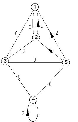
CYCLIC COVERINGS Each semiregular symmetry allows us to regard the graph as a cyclic covering of some smaller graph. If the symmetry includes the cycles (u_0, u_1, u_2, . . . u_n-1)(v_0, v_1, v_2, . . . v_n-1) and {u_0, v_a} is an edge, then every {u_i, v_a+i} is an edge, and we can make a graph including the vertices u and v and the label a on the directed edge (u, v). On the Constructions page for each graph, and for each such symmetry, we provide such a diagram in the form of a skew-symmetric matrix of sets of numbers mod n. The numbers in row u, column v are all the weights of edges from u to v.
For example, the matrix:
| 1 | 2 | 3 | 4 | 5 | |
|---|---|---|---|---|---|
| 1 | - | 0 5 | 0 | - | 4 |
| 2 | 0 1 | - | 0 | - | 5 |
| 3 | 0 | 0 | - | 0 | 0 |
| 4 | - | - | 0 | 2 4 | 0 |
| 5 | 2 | 1 | 0 | 0 | - |
Stands for the diagram:
OTHER COVERINGS When one graph in this Census is a covering of another, the fact is listed on the Related Graphs page of each of the two graphs, including a link to the other graph's summary page. Note that not all covering are found here. We show only those coverings that result from a system of imprimitivity of some subgroup of the full symmetry group.
Aut-orbital Graphs Given a graph Γ and its symmetry group G = Aut(Γ), and given any two vertices u and v, we can construct a new graph having the same vertices as the old, and using the orbit of {u,v} as the set of edges. If the result is disconnected, we take any one component. All such graphs are shown on the Related Graphs page for Γ.
BGCG dissections When a graph Γ admits a BGCG dissection with base graph B and connection graph C, this fact is noted on the Related Graphs pages for both Γ and B. When the graph C is easy to recognize, we name it. Otherwise, we give the order and valence of the graph.