


 |
 |
 |
 |
  |
|
§ Excel and Equations §
Excel- commands used in this topic (Excel in Office 97 and Office 2000)

§ Equations §
Excel Steps
Frequency Distributions
(1) Use the steps to get a histogram. The frequency distribution will be a part of that output. Click on Tools-Data Analysis-Histograms. If Data Analysis does not show up, then click on Tools-Addins and select the top two options of Analysis Pack and Analysis Pack VBA.


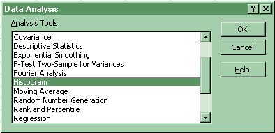

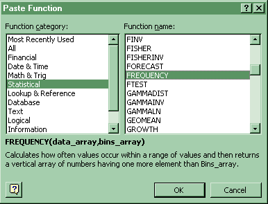
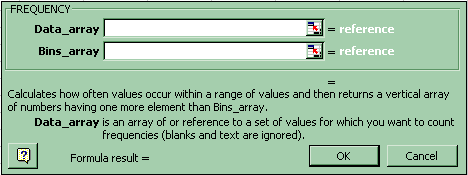
(2) Create Bin value equal to the upper class limit (UCL) of each class. Highlight the cells next to the Bin values plus one cell. Click Paste-Function-Statistical-Frequency. Fill in the arrays in the box. While the box is still opend press Control-Shift-Enter.
![]()
Poisson Distribution
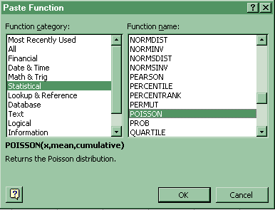
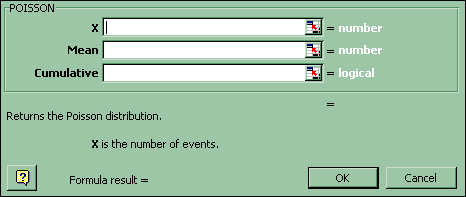
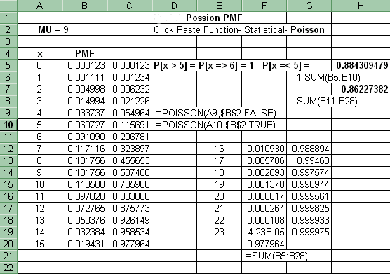
Click the Paste Function-Statistical-Poisson
![]()
Discrete Probability
Equations
Discrete Probability Equations used at this web site
§ Probability §
§ Discrete random variable § Population Mean §
§ Conceptual Variance and Standard Deviation §
§ Computing Variance and Standard Deviation §
§ Poisson PMF § Other Discrete Probability Equations §
§ Other Probability and Counting Rules §
1. Probability
Probability of event A = P(A) = m / n
where,
(a) The ratio m / n is a relative frequency.
(b) m = total number of times a single outcome occurs in an experiment
(c) n = total number of outcomes possible in an experiment
2. Discrete random variable.
X (random variable) = x1 with P(x1) or
= x2 with P(x2) or
= ... or
= ... or
= xn with P(xn)
n = the number of possible outcomes in the experiment.
0 £ P(xn) £ 1
SP(xn) = 1
3. Population Mean
The population mean for any discrete probability distribution:
m = SxiP[xi]
4. Conceptual Variance and Standard Deviation
Conceptual formulae for the variance and standard deviation for any discrete probability distribution:
(a) variance
s² = S[xi - m]²( P[xi] ) (do not use for hand calculations)
(b) standard deviation
s = Ös² = Ö(S[xi - m]²( P[xi] ) (do not use for hand calculations)
5. Computing Variance and Standard Deviation
Computing formulae for the variance and standard deviation for any discrete probability distribution:
(a) variance
s² = Sxi²P[xi] - m² ( use for hand calculations)
(b) standard deviation
s = Ös² = Ö (Sxi²P[xi] - m²) ( use for hand calculations)
6. Poisson PMF
P[x] = [mx][e - m] / x! (Do not use for hand calculations. Use table.)
where x = expected number of occurrences over time
and e = 2.71828...
(a) m = SxiP[xi]
(b) s² = Sxi²P[xi] - m²
(c) m = s²
Other Discrete Probability Equations not covered at this web site
§ Binomial PMF § Hypergeometric PMF §
§ Other Probability and Counting Rules §1. Binomial PMF:
P[xi] = nCx(px)(1 - p)(n - x)
n = # trials)
x = # of success = # tails
p = probability of success
nCx = n! / [x!(n - x)!]
2. For the Binomial Random Variable:
(a) Binomial Mean
m = SxiP[xi] = n( p )
(b) Binomial Variance
s² = Sxi²P[xi] - m² = n( p )[1 - p]
n = # trials)
x = # of success = # tails
p = probability of success
3. Hypergeometric PMF:
P[x] = {[kCx][ (N - k)C(n - x) ]} / NCn
(a) kCx is the number of successes, x out of k possible successes.
(b) N - k)C(n - x) is the number of failures ( n - x ) out of ( N - k) possible failures.
(c) NCn is the number of samples n out of a finite population size N.
<####) Mean
m = SxiP[xi] = nk / N
(e) Variance
s² = Sxi²P[xi] - m²
= [n(k/n)(1- {k/N})] x [( N - n )/( N - 1)]
where[(N - n)/(N - 1)] = the finite population correction (fpc) factor
Other Probability and Counting Rules not covered at this topic site
§ Complement of an Event § Additive Rule §
§ Mutually Exclusive § Multiplicative Rule §
§ Independent Events § Rules for Conditionals § Counting Rules §
§ Combinations and Samples from a Population §
1. Complement of an Event:
P(A) + P(notA) = 1
P(A) = 1 - P(notA)
P( notA) = 1 - P(A)
2. Additive Rule:
The "or" probability (union)
P[A or B] = P(A) + P(B) - P(A & B)
3. Special Case of the Additive Rule:
Mutually Exclusive
P[A or B] = P(A) + P(B)
4. Multiplicative Rule:
The "and" probability (intersection)
P[A & B] = P[ A | B ]P[B]
= P[ B | A ]P[A]
5. Special Case of the Multiplicative Rule:
Independent Events
P[A|B] = P[ A ]
P[B|A] = P[ B ]
P[A & B] = P[ A ]P[ B]
6. Rules for Conditionals:
P[A | B] = P[ A & B ] / P[ B ], for P[B] > 0
P[B | A] = P[ A & B ] / P[ A ], for P[A] > 0
7. Counting Rules:
(a) Filling Slots k different independent slots. (Counting Rule # 1)
(n1)(n2)(...)(nk)
(b) Permutations (Counting Rule # 2):
nPk = [n!] / [n - k]! = (n)(n - 1)(n - 2)(...)(n - k - 1)
n is the total number of objects
k is the number of objects selected
Used when order is important.
(c) Combinations (Counting Rule # 3):
nCk = [ nPk ] / k! = [n!] / [k!][n - k]!]
n is the total number of objects
k is the number of objects selected
Used when order is not important.
8. The total numberof samples possible of size n, selected without replacement from a population size N is:
Combinations and Samples from a Population
NCn = [N!] / [n!][N - n]!,
probability of any one sample selected 1 / NCn
Go on to
Home Work
or
Go back to Discrete
Distributions: Activities and Assignments
Please reference "BA501 (your last name) Assignment name and number" in the subject line of either below.
E-mail Dr. James V. Pinto at
BA501@mail.cba.nau.edu
or call (928) 523-7356. Use WebMail for attachments.

Copyright 2002 Northern Arizona University
ALL RIGHTS RESERVED