Introduction: Multi-dimensional Data Access Methods
Multi-dimensional data access methods are used to reduce the complexity of brute force range queries. For a given range query, instead of comparing all $|D|$ data points to the ranges in each dimension, a spatial partitioning of the dataset can be used to reduce the number of comparisons between points and the ranges in each dimension. In this module, we will index $D$ using the R-tree. Note that there are other spatial indexing methods that could be employed, such as kd-trees, quad-trees, oct-trees, ball trees, and others.
Optional Reading
- Guttman, A. R-trees: a dynamic index structure for spatial searching. In Proc. of the 1984 ACM SIGMOD Intl. Conf. on Management of Data pp 47-57. [link]
R-tree Overview
An R-tree (Rectange-tree) stores objects in rectangles (here, objects refer to our data points in $D$). The main idea of the R-tree is to construct the index using a hierarchy of bounding rectangles as a function of the input data. The root of the tree contains the entire dataset, and as the tree is traversed, there are fewer objects that overlap a given range query.
Figure 3 outlines an example of indexing data in an R-tree. The input data objects refer to the red rectangles, $R8, R9, \ldots, R19$. The rectangles $R1, R2, \ldots, R7$ are internal rectangles and are constructed based on the input data objects. As an example, observe that to find $R16$, the tree is traversed as follows: $R2 \rightarrow R6 \rightarrow R16$. Therefore, for a given range query, the data is partitioned based on the distribution of the internal rectanges ($R1, R2, \ldots, R7$) which avoid making a comparison to all points in $D$ (unless the range is sufficiently large in all dimensions).
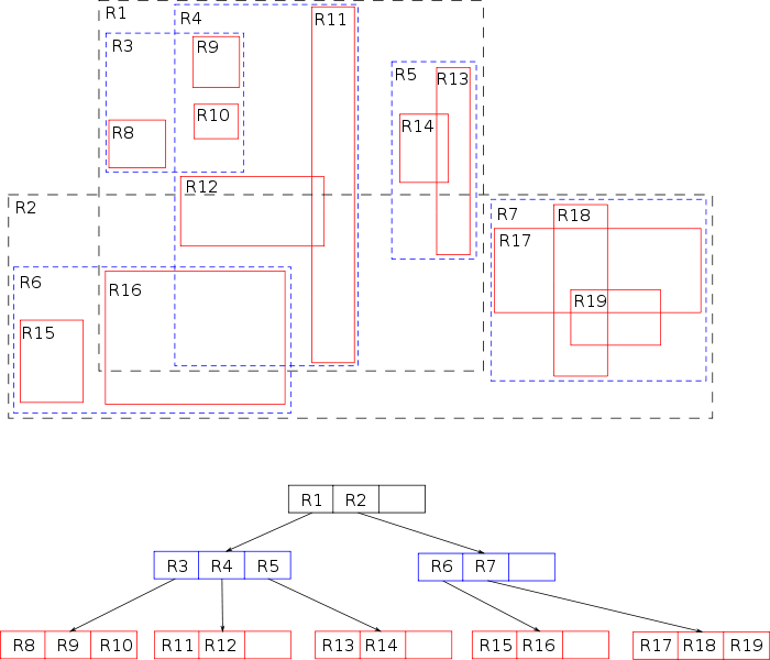
Figure 3: Example R-tree. Image: Public domain.
R-tree Indexing
R-trees index data objects and search using minimum bounding rectanges (MBRs). That is why in Figure 3, the data objects $R8,\ldots,R19$ are shown as rectangles (and not points as shown in Figure 2). A data object is defined using the minimum and maximum values of the MBR (Figure 4). Let $m$ be a 2-dimensional MBR, which is defined as follows:
$$m=(x^{min}, y^{min}, x^{max}, y^{max}).$$

Figure 4: Example Minimum Bounding Rectangle (MBR).
For a 2-D point object that does not have a spatial extent, note that $x^{min}=x^{max}$ and $y^{min}=y^{max}$. Therefore, if $p_x$ and $p_y$ denote the $x$ and $y$ coordinates of a point, then the MBR for this point is defined as follows: $m=(p_x, p_y, p_x, p_y)$. To construct an R-tree index, data is inserted as MBRs into the tree.
R-tree Searching
After indexing data in an R-tree, you simply define a range query using an MBR as described above, which outlines the minimum and maximum ranges in each dimension. Then search the R-tree using this MBR.
Tutorial: Using an R-tree
During this miniature tutorial, follow along using range_query_rtree_100ZTF_objects_example.cpp. We will search the first 100 data points shown in Figure 1, which are shown in Figure 5.

Figure 5: A sample of 100 data points from Figure 1. There are 5 objects found by the range query.
- Download the files
range_query_rtree_100ZTF_objects_example.cppandRTree.h. RTree.hhas been downloaded from superliminal.com from here. I have made a few minor modifications to the file to remove compiler errors and warnings under g++ (tested using v.4.4.7 and v.5.4.0). This R-tree implementation has been used extensively by the community.
The R-tree uses C++ and is templated. To compile, use C++ (not C) using the following command:
mpic++ -O3 range_query_rtree_100ZTF_objects_example.cpp -lm -o range_query_rtree_100ZTF_objects_example
The file will import all of the data in Figure 5 (the first 100 objects in Figure 1).
The line that constructs the R-tree is as follows.
RTree<int, double, 2, double> tree;
The four parameters are: <DATATYPE> <ELEMTYPE> <NUMDIMS> <ELEMTYPEREAL>, and are described as follows:
- <DATATYPE>: The type of the reference data (object 1, 2, 3).
- <ELEMTYPE>: The type of the data that will be indexed (RA/Dec).
- <NUMDIMS>: The dimensionality of the data (2 dimensions).
- <ELEMTYPEREAL>: Data type used in volume calculations (use a double to minimize floating point error).
To construct the R-Tree, create MBRs from the data. The lines that perform this task are below:
for (int i=0; i<N; i++)
{
    Rect tmp=Rect(data[i].x,data[i].y,data[i].x,data[i].y);
    tree.Insert(tmp.min, tmp.max, i);
}
To search the R-tree for the MBR shown in Figure 1, we create an MBR and search the tree, using the lines below:
Rect search_rect=Rect(150.0, 0.0, 190.0, 30.0);
unsigned int nhits=tree.Search(search_rect.min, search_rect.max, MySearchCallback, NULL);

//The value of nhits is the number of objects within the MBR, which returns 5 objects.
Programming Activity #2
Implement the range query algorithm using the instructions outlined in Programming Activity #1, but use an R-tree. Note the following:
- Use
range_query_rtree_starter.cpp. The starter file is the same asrange_query_starter.c, except that it has the.cppextension and includesRTree.h. - Remember to compile using
mpic++.
Similarly to Programming Activity #1, complete the following tables using one node. Note that your global sum should be identical to your brute force implementation for a given value of $p$. The R-tree implementation has an index construction phase and a search phase. Time the following components:
- The total response time (maximum time across all ranks).
- The time to construct the R-tree (maximum time across all ranks).
- The time to perform the searches (maximum time across all ranks).
Table 2: Total response time, index construction time, and search time (one node).
| # of Ranks ($p$) | Total Time (s) | R-Tree Construction (s) | Search Time (s) | Global Sum | Job Script Name (*.sh) |
|---|---|---|---|---|---|
| 1 | |||||
| 4 | |||||
| 8 | |||||
| 12 | |||||
| 16 | |||||
| 20 |
Table 3: Speedup and parallel efficiency of the search phase from Table 2.
Typically, databases are indexed once and then queried multiple times. Therefore, index construction time can be disregarded. Compute the speedup and parallel efficiency using the index search time (not total response time) from Table 2.
| # of Ranks ($p$) | Speedup | Parallel Efficiency |
|---|---|---|
| 1 | ||
| 4 | ||
| 8 | ||
| 12 | ||
| 16 | ||
| 20 |
Using the data you collected in your tables, answer the following questions. Be sure to refer to specific values in your tables when responding to these questions.
- Q3: Each rank constructs an identical R-tree but searches the index for different range queries. How does the time to construct the index change with increasing $p$? Explain this performance behavior.
- Q4: Which implementation has better performance, the R-tree (search only time) or the brute force algorithm? Explain.
- Q5: Which has the highest parallel efficiency, the brute force algorithm or the R-tree? Why do you think the parallel efficiency varies between algorithms?